So we reached a good point, we can span and manage virtual machines, we can start simulations, and we can connect the machines to the simulations. Seems like everything is well and done, right? Not even close. While what we did so far works, its results aren’t reliable at all.
Problem with Time
The problem we faced at that point was that network channel simulations are expensive. They take significantly longer than transmissions over real channels. What even complicates things further is how sensitive they’re to network load. Their performance varies a lot throughout a single scenario. So what are the implications of that:
- Reading by the virtual machines are very inacurate
- Timeouts
- TCP congestion control
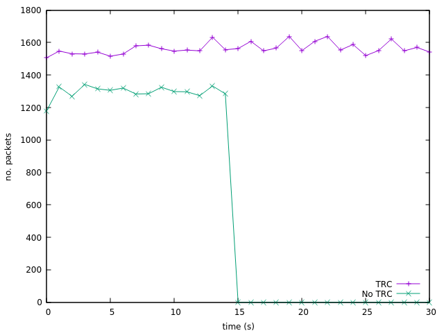
The first two issues are straightforward, but the congestion control part is a bit tricky if you’re not familiar with how TCP works. This is out of the scope of this article but you can read more about congestion control and it’ll make sense. But to summarize, packet retranmissions, timeouts, and latency in general can affect the performance of ac TCP connection as it adjusts to the network. To show the effect of having time rate control on the scenario itself, check this figure

This figure is for a 30-second transfer of packets over a network with no other traffic or noise. Two things we notice here: 1. the connection was dropped halfway through, 2. the reported performance was lower than that of the time-rate-controlled traffic. This is even aggrevated in more realistic scenarios.
So we needed a way to make time inside the virtual machines move at the same rate as the simulation. And that’s what we’re about to do.
The Naive Approach
So the first solution that came to mind was very sophisticated. What if we had a tool which runs in every machine and compares the latency against some baseline and then a concensus algorithm to make sure that they all agree on the rate. Being someone who likes distributed systems, I liked that solution, and naively I was proud of it and excited to implement it. The main problem with that is how complicated it is. It also adds another stream of data which contributes nothing to the scenario, essentially adding traffic noise which isn’t built into the scenario itself.
The Better Approach
While trying to improve the naive approach, I remembered something quite crucial: ns3 is a discrete event simulator. The implication is that the simulation time moves in consistent blocks (intervals). So the better solution was to have a component running in the background, which keeps an eye on the simulation time intervals and compares them to the real time elapsed.
Calculating Time Rate Difference
Time rate is represented as an integer percentage; value of 200 causes time to move two times slower, while a value of 50 causes it to move twice as fast. Time rate at a particular moment is calculated as R = E s / E r × 100. Where Es is the elapsed simulation time, and Er is the elapsed real time.
Time rate values are prone to flunctuations and unusual spikes. Therefore, the previous equation should be used to calculate a new time rate Ri based on the current time rate R, the previous time rate Ri−1, the list of previous non-smoothed R values, and the number of values so far n.
Ri = smooth(Ri−1 , R, RL , n)
The role of the smooth function is to prevent momentary spikes and flunctuations. It could also only allow time rate to move in only a single direction, i.e. only decreasing. Or change it only if the change crossed a certain threshold. There are many options to use for that function but the two which made the scenarios be most realistic were comulative average and simple moving average.
Applying the Time Rate
This was another are where I had a couple of naive solutins, including modifying the linux kernel itself. But thankfully, I was sane at that time enough to find more managable solutins. After going through VirtualBox developer documentation I stumbled upon a debugging features which allows something to change the time rate of the virtual clock of a machine.
Conclusion
That was probably one of the weirdest features I’ve ever worked on, and still one of the most fun and challenging ones. Now we have a complete solutions, but it has its own drawbacks too. In the next, and final, part I’ll then talk about the modifications I had planned for version 2.0 of the platform but never got to implement.